Functions for Plotting and Analysis
Source:vignettes/Plotting_And_Analysis.Rmd
Plotting_And_Analysis.Rmd
Sys.setenv(OMP_THREAD_LIMIT = 1) # Reducing core use, to avoid accidental use of too many cores
library(Colossus)
library(data.table)
#>
#> Attaching package: 'data.table'
#> The following object is masked from 'package:base':
#>
#>     %notin%
if (system.file(package = "survival") != "") {
  library(survival)
}
library(dplyr)
#>
#> Attaching package: 'dplyr'
#> The following objects are masked from 'package:data.table':
#>
#>     between, first, last
#> The following objects are masked from 'package:stats':
#>
#>     filter, lag
#> The following objects are masked from 'package:base':
#>
#>     intersect, setdiff, setequal, union
if (system.file(package = "ggplot2") != "") {
  library(ggplot2)
}
Example Setup
We will use analysis of the lung dataset in the survival package to visualize the different plotting methods available in Colossus.
if (system.file(package = "survival") != "") {
  data(cancer, package = "survival")
  cancer |> setDT()
  df <- copy(cancer)
} else {
  status <- c(2, 2, 1, 2, 2, 1, 2, 2, 2, 2, 2, 2, 2, 2, 2, 2, 2, 2, 2, 2, 2, 2, 2, 2, 2, 2, 2, 2, 2, 2, 2, 2, 2, 2, 2, 2, 2, 1, 2, 2, 2, 2, 2, 2, 2, 2, 2, 2, 2, 2, 2, 2, 2, 2, 2, 2, 2, 2, 2, 2, 2, 2, 2, 2, 2, 2, 2, 1, 2, 2, 1, 2, 2, 2, 2, 2, 2, 2, 2, 2, 2, 2, 1, 2, 1, 2, 2, 2, 1, 2, 2, 2, 2, 2, 1, 2, 2, 2, 2, 2, 1, 2, 2, 2, 2, 2, 1, 2, 2, 2, 2, 2, 2, 2, 2, 2, 2, 2, 2, 2, 2, 2, 2, 2, 2, 2, 2, 2, 1, 1, 2, 2, 2, 1, 2, 1, 2, 2, 2, 2, 2, 1, 2, 2, 1, 1, 2, 2, 2, 2, 2, 1, 1, 2, 2, 2, 1, 2, 2, 1, 1, 2, 1, 2, 1, 1, 2, 2, 2, 2, 1, 2, 2, 1, 1, 1, 2, 2, 2, 1, 1, 1, 2, 1, 1, 1, 2, 1, 2, 2, 2, 2, 2, 1, 2, 1, 1, 1, 1, 2, 2, 2, 1, 1, 1, 2, 1, 2, 1, 1, 1, 1, 1, 1, 2, 1, 1, 2, 1, 1, 1, 1, 2, 1, 1, 1, 1, 1)
  sex <- c(1, 1, 1, 1, 1, 1, 2, 2, 1, 1, 1, 2, 2, 1, 1, 1, 1, 1, 2, 1, 1, 2, 1, 1, 1, 2, 1, 1, 1, 1, 2, 1, 1, 2, 1, 2, 1, 2, 1, 2, 1, 2, 2, 2, 1, 2, 1, 1, 1, 2, 2, 1, 1, 1, 1, 1, 2, 1, 2, 2, 2, 1, 1, 2, 1, 1, 2, 2, 1, 1, 1, 2, 1, 1, 2, 2, 2, 2, 1, 1, 1, 1, 1, 2, 1, 1, 2, 1, 2, 1, 1, 1, 1, 2, 2, 1, 1, 1, 1, 2, 2, 2, 1, 1, 1, 1, 2, 1, 1, 2, 1, 1, 1, 2, 2, 1, 1, 1, 1, 1, 1, 2, 2, 1, 1, 1, 1, 1, 2, 2, 2, 1, 1, 2, 1, 2, 2, 1, 1, 1, 2, 1, 1, 2, 1, 2, 1, 1, 1, 2, 1, 1, 2, 2, 1, 1, 2, 1, 1, 2, 2, 2, 1, 1, 1, 2, 2, 1, 1, 1, 1, 2, 1, 2, 1, 2, 1, 2, 2, 2, 1, 1, 2, 2, 2, 2, 2, 1, 1, 1, 1, 1, 1, 1, 1, 1, 2, 1, 2, 1, 2, 1, 2, 2, 2, 1, 2, 2, 1, 2, 2, 1, 1, 2, 1, 1, 2, 1, 2, 2, 1, 2, 1, 1, 1, 2, 1, 2)
  time <- c(306, 455, 1010, 210, 883, 1022, 310, 361, 218, 166, 170, 654, 728, 71, 567, 144, 613, 707, 61, 88, 301, 81, 624, 371, 394, 520, 574, 118, 390, 12, 473, 26, 533, 107, 53, 122, 814, 965, 93, 731, 460, 153, 433, 145, 583, 95, 303, 519, 643, 765, 735, 189, 53, 246, 689, 65, 5, 132, 687, 345, 444, 223, 175, 60, 163, 65, 208, 821, 428, 230, 840, 305, 11, 132, 226, 426, 705, 363, 11, 176, 791, 95, 196, 167, 806, 284, 641, 147, 740, 163, 655, 239, 88, 245, 588, 30, 179, 310, 477, 166, 559, 450, 364, 107, 177, 156, 529, 11, 429, 351, 15, 181, 283, 201, 524, 13, 212, 524, 288, 363, 442, 199, 550, 54, 558, 207, 92, 60, 551, 543, 293, 202, 353, 511, 267, 511, 371, 387, 457, 337, 201, 404, 222, 62, 458, 356, 353, 163, 31, 340, 229, 444, 315, 182, 156, 329, 364, 291, 179, 376, 384, 268, 292, 142, 413, 266, 194, 320, 181, 285, 301, 348, 197, 382, 303, 296, 180, 186, 145, 269, 300, 284, 350, 272, 292, 332, 285, 259, 110, 286, 270, 81, 131, 225, 269, 225, 243, 279, 276, 135, 79, 59, 240, 202, 235, 105, 224, 239, 237, 173, 252, 221, 185, 92, 13, 222, 192, 183, 211, 175, 197, 203, 116, 188, 191, 105, 174, 177)
  age <- c(74, 68, 56, 57, 60, 74, 68, 71, 53, 61, 57, 68, 68, 60, 57, 67, 70, 63, 56, 57, 67, 49, 50, 58, 72, 70, 60, 70, 53, 74, 69, 73, 48, 60, 61, 62, 65, 66, 74, 64, 70, 73, 59, 60, 68, 76, 74, 63, 74, 50, 72, 63, 68, 58, 59, 62, 65, 57, 58, 64, 75, 48, 73, 65, 69, 68, 67, 64, 68, 67, 63, 48, 74, 40, 53, 71, 51, 56, 81, 73, 59, 55, 42, 44, 44, 71, 62, 61, 44, 72, 63, 70, 66, 57, 69, 72, 69, 71, 64, 70, 58, 69, 56, 63, 59, 66, 54, 67, 55, 75, 69, 44, 80, 75, 54, 76, 49, 68, 66, 80, 75, 60, 69, 72, 70, 66, 50, 64, 77, 48, 59, 53, 47, 55, 67, 74, 58, 56, 54, 56, 73, 74, 76, 65, 57, 53, 71, 54, 82, 59, 70, 60, 62, 53, 55, 69, 68, 62, 63, 56, 62, 44, 69, 63, 64, 57, 60, 46, 61, 65, 61, 58, 56, 43, 53, 59, 56, 55, 53, 74, 60, 39, 66, 65, 51, 45, 72, 58, 64, 53, 72, 52, 50, 64, 71, 70, 63, 64, 52, 60, 64, 73, 63, 50, 63, 62, 55, 50, 69, 59, 60, 67, 69, 64, 65, 65, 41, 76, 70, 57, 67, 71, 76, 77, 39, 75, 66, 58)

  df <- data.table(
    status = status,
    sex = sex,
    time = time,
    age = age
  )
}

df$UserID <- seq_len(nrow(df))

df$status <- df$status - 1

control <- list(ncores = 1)
a_n <- c(0.01701289, -0.51256478)
coxres <- CoxRun(Cox(time, status) ~ loglinear(age, sex, 0),
  df,
  control = control, a_n = a_n
)
In general the plot.coxres() function can be used to
call the various different types of plots using a list of plotting
options. In this vignette we will be calling the specific functions for
each application.
Survival Function Approximation
After fitting a Cox proportional hazards model, one may be interested in what the baseline survival rate is. One method of doing so is by weighting the number of events at each event time by the total hazard ratio. In the absence of excess risk, the hazard at any point in time is equal to the event rate and the hazard ratio of every row is equal to one, so this assumption holds for the case with negligible excess risk.
Suppose every row at risk at a time was twice as likely to experience
an event than the baseline. Then we would expect there to be twice as
many events as there would be at baseline. The same logic applies to the
case with every row at risk being half as likely. This generalizes to
any average risk. Colossus allows the instantaneous hazard
to be approximated for both stratified and non-stratified models.
Once the instantaneous hazard is approximated, the cumulative hazard can be approximated. Then the surviving fraction is approximately equal to the exponential of the negative cumulative hazard at each event time.
We can calculate the instantaneous hazard, cumulative hazard, and baseline surviving fraction using the ’plotSurvival.coxres()` function. We can get the Kaplan-Meier estimates using the KM option.
# We can start by obtaining the approximated survival curve data
plot_options <- list(
  studyid = "UserID",
  verbose = 2, surv_curv = TRUE
)

# We apply it to a regression solution
e <- plotSurvival(coxres, df, plot_options)

# The results include both the standard and log results:
# hazard, cumulative hazard, and survival curves

norm_surv <- e[["standard"]]

# The time is named 't'
# The instantaneous hazard is 'h'
if (system.file(package = "ggplot2") != "") {
  g <- ggplot(norm_surv, aes(x = .data$t, y = .data$h)) +
    geom_point(color = "black") +
    labs(x = "age", y = "Instantaneous Hazard")
} else {
  g <- message("ggplot2 wasn't detected. Please install to see the plot")
}
g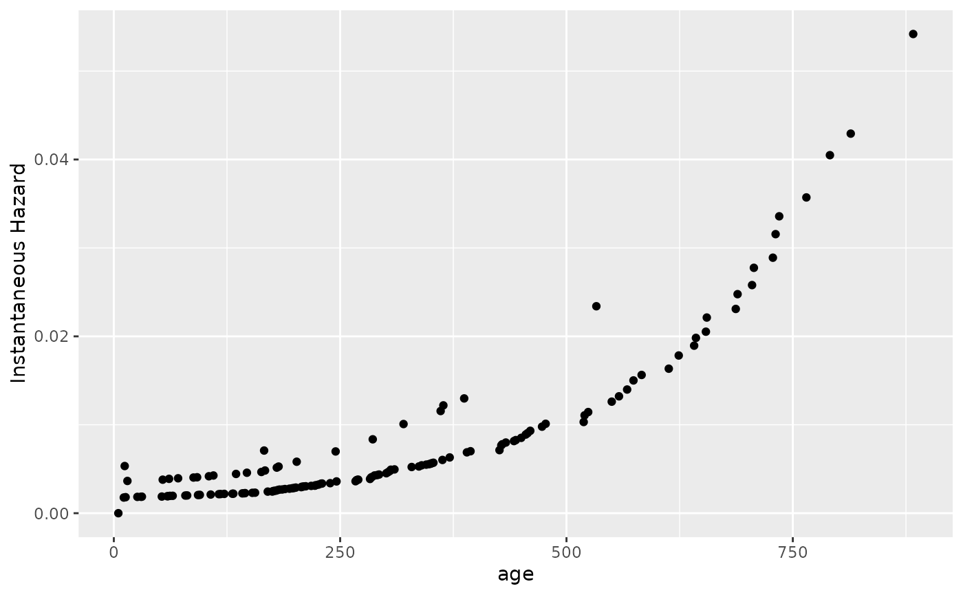
# The cumulative hazard is 'ch'
if (system.file(package = "ggplot2") != "") {
  g <- ggplot(norm_surv, aes(x = .data$t, y = .data$ch)) +
    geom_line(color = "black", alpha = 1) +
    labs(x = "age", y = "Cumulative Hazard")
} else {
  g <- message("ggplot2 wasn't detected. Please install to see the plot")
}
g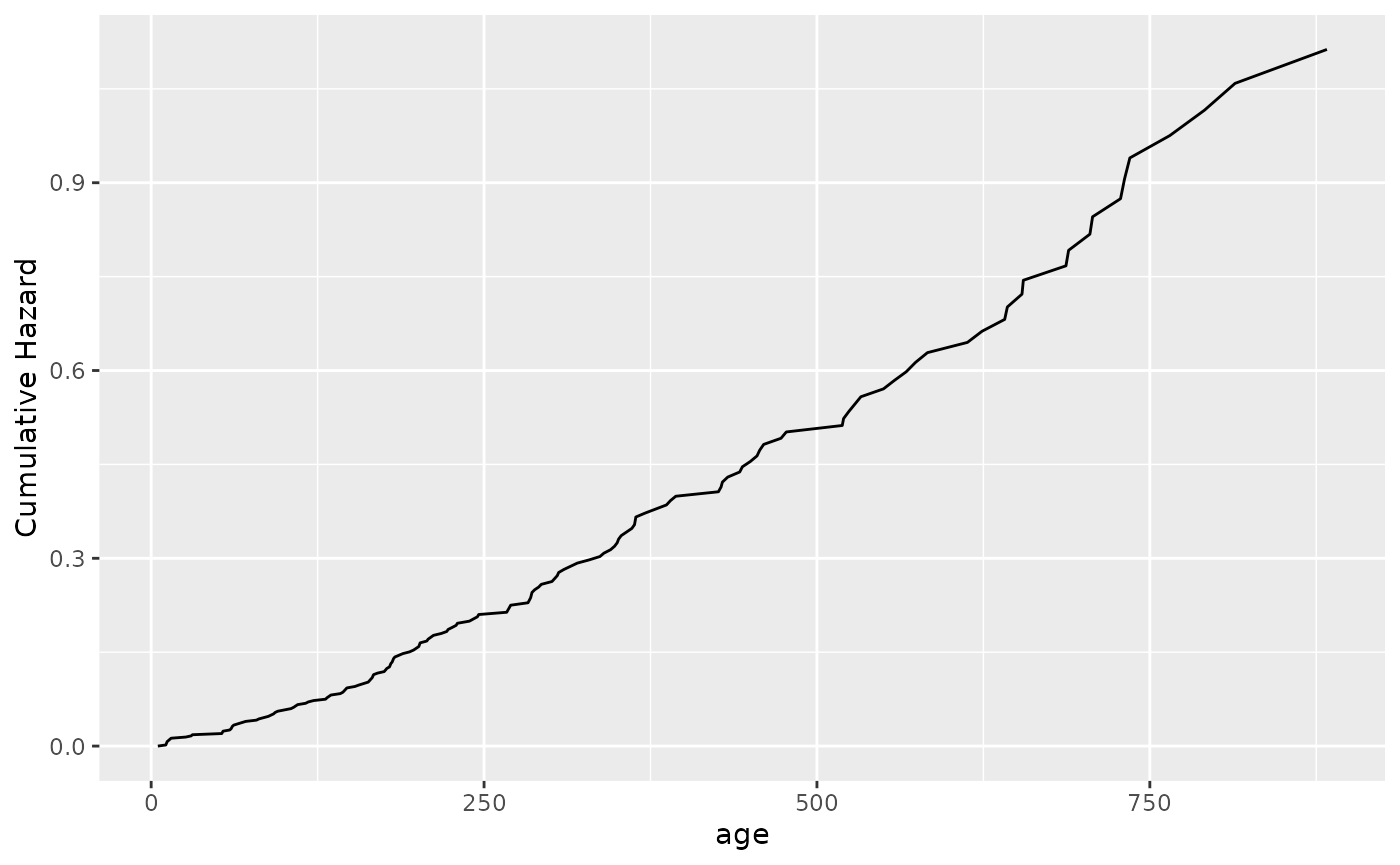
# The surviving fraction is 'surv'
if (system.file(package = "ggplot2") != "") {
  g <- ggplot(norm_surv, aes(x = .data$t, y = .data$surv)) +
    geom_line(color = "black", alpha = 1) +
    labs(x = "age", y = "Surviving Fraction")
} else {
  g <- message("ggplot2 wasn't detected. Please install to see the plot")
}
g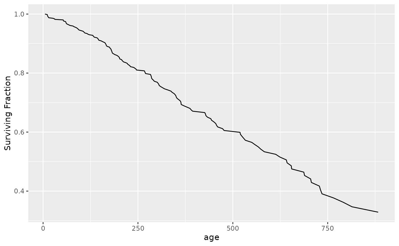
# We might also want to find the kaplan-meier estimate
plot_options <- list(
  studyid = "UserID",
  verbose = 2, km = TRUE
)

e <- plotSurvival(coxres, df, plot_options)
# Multiple results can be returned at once.
# In this case, the result is the "kaplan-meier" value.
km <- e[["kaplin-meier"]]
# The survival curve is the 'n_t' value
if (system.file(package = "ggplot2") != "") {
  g <- ggplot(km, aes(x = .data$t_t, y = .data$n_t)) +
    geom_line(color = "black", alpha = 1) +
    labs(x = "age", y = "KM Survival")
} else {
  g <- message("ggplot2 wasn't detected. Please install to see the plot")
}
g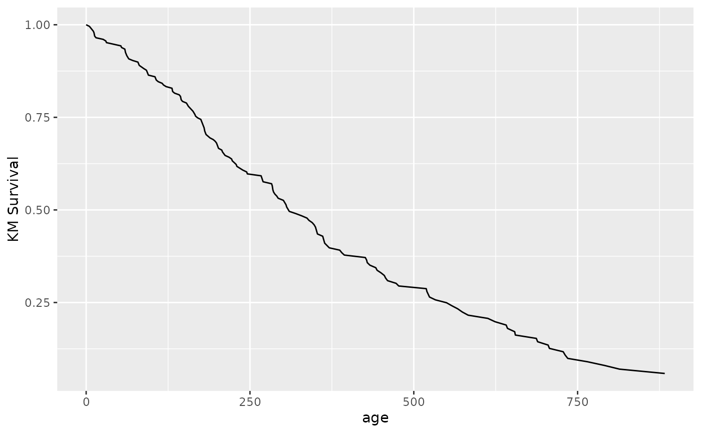
t_total <- c(norm_surv$t, km$t_t)
surv_total <- c(norm_surv$surv, km$n_t)
method <- c(rep("adjusted", nrow(norm_surv)), rep("km", nrow(km)))

comp_plot <- data.table(t = t_total, y = surv_total, method = method)
# Plot them combined
if (system.file(package = "ggplot2") != "") {
  g <- ggplot(comp_plot, ggplot2::aes(x = .data$t, y = .data$y, group = .data$method, color = .data$method)) +
    geom_line(alpha = 1, linewidth = 1.2) +
    labs(x = "age", y = "Survival")
} else {
  g <- message("ggplot2 wasn't detected. Please install to see the plot")
}
g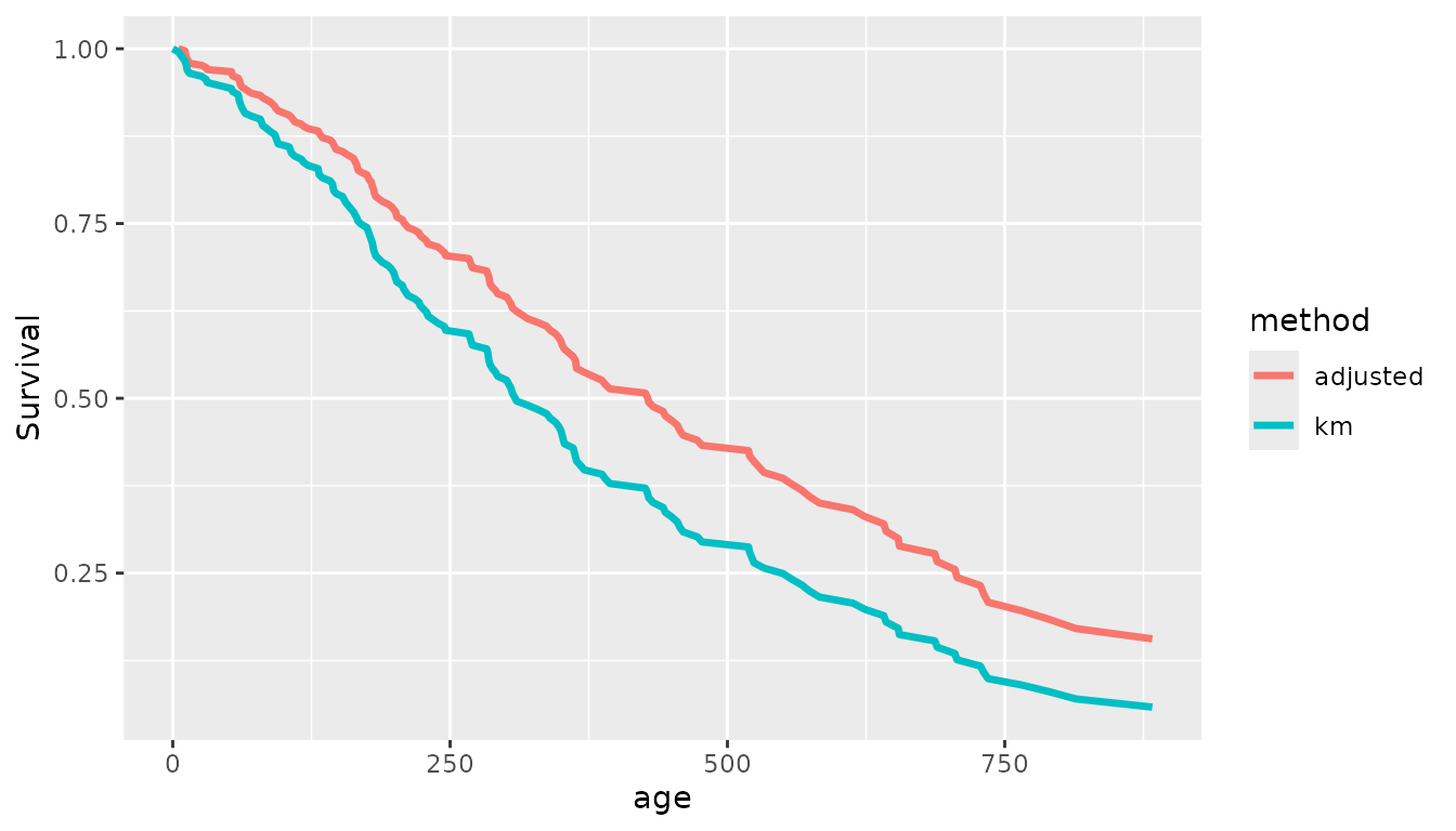
Cox Proportional Hazards model assumptions
The Cox proportional hazards model by definition assumes proportional
hazards independent of time. If this is violated, then the results of a
regression may be misleading. There are two checks that
Colossus provides that can be used to test this assumption,
the Schoenfeld residuals and Martingale residuals. In both cases, the
premise is that if the hazard ratio were independent of time, then the
residuals should also be independent of time.
Schoenfeld Residuals
Schoenfeld residuals compare the average covariate value of rows with events with the risk-weighted average of the covariate in rows at risk. Consistently high or low residuals may be due to the hazard being much higher or lower than the model predicts. If these residuals are also correlated with event time, then the hazard ratio may be dependent on event time. There is also the option to scale the residuals by the standard deviation.
We can plot schoenfeld residuals using the
plotSchoenfeld.coxres() function.
plot_options <- list(
  studyid = "UserID", verbose = 2
)

res_all <- plotSchoenfeld(coxres, df, plot_options)
# results are produced for every covariate
res_age <- res_all[["age"]]
if (system.file(package = "ggplot2") != "") {
  g <- ggplot(res_age, aes(x = .data$time, y = .data$y)) +
    geom_point(color = "black") +
    labs(
      x = paste("Survival Time", sep = ""),
      y = paste("Schoenfeld Residual (age)", sep = " ")
    )
} else {
  g <- message("ggplot2 wasn't detected. Please install to see the plot")
}
g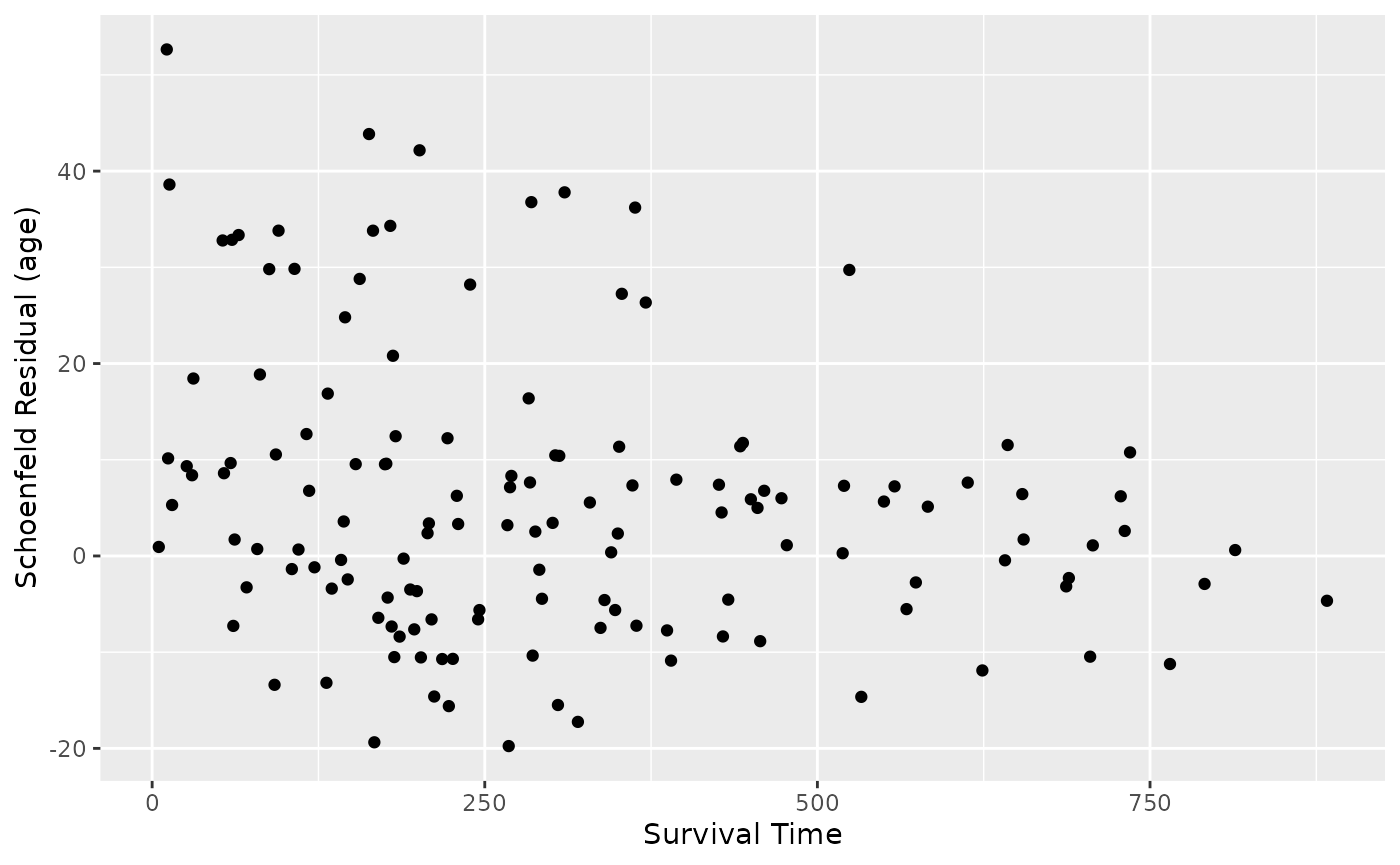
if (system.file(package = "ggplot2") != "") {
  g <- ggplot(res_age, aes(x = .data$time, y = .data$y_scale)) +
    geom_point(color = "black") +
    labs(
      x = paste("Survival Time", sep = ""),
      y = paste("Schoenfeld Residual Scaled (age)", sep = " ")
    )
} else {
  g <- message("ggplot2 wasn't detected. Please install to see the plot")
}
g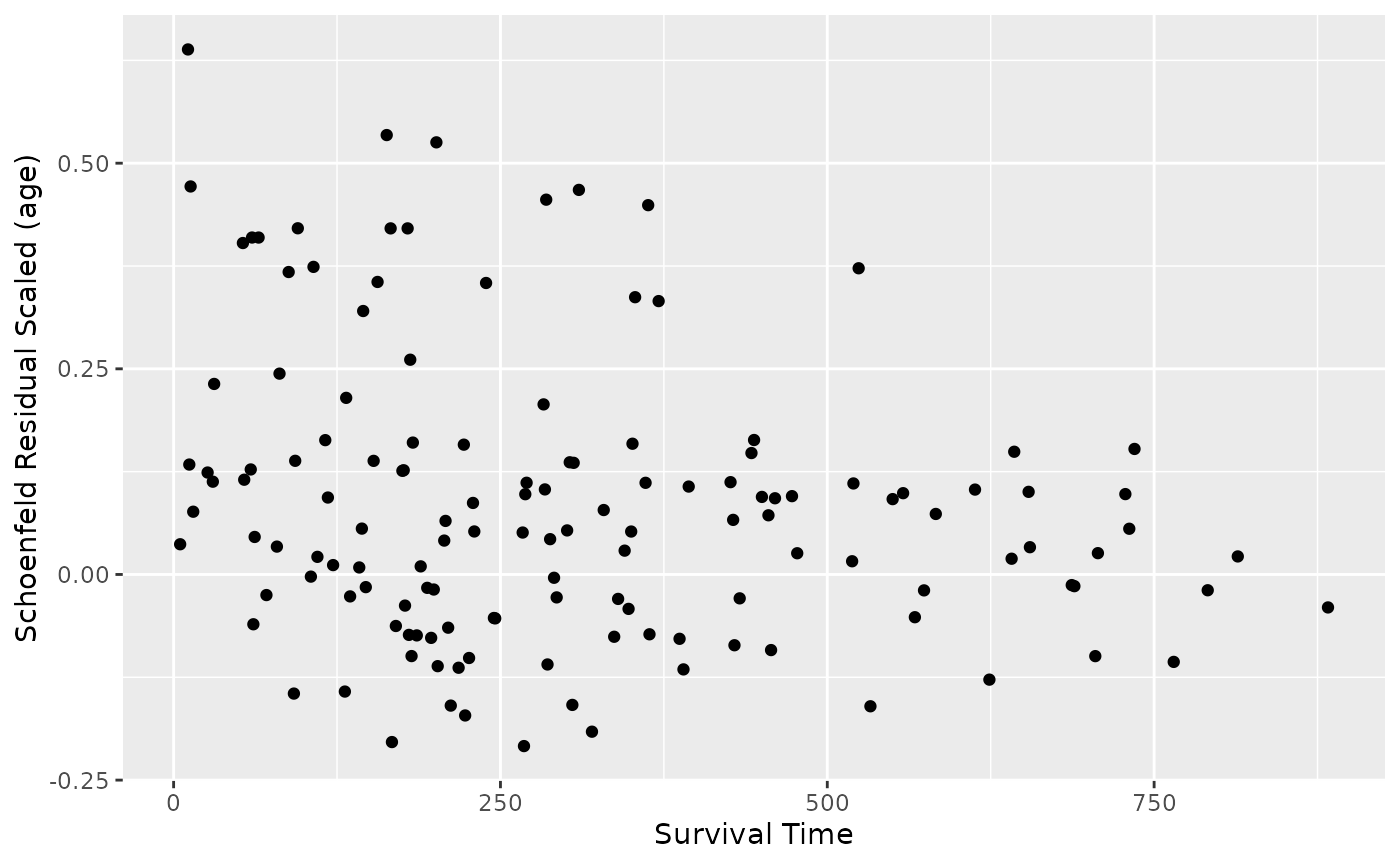
res_sex <- res_all[["sex"]]

if (system.file(package = "ggplot2") != "") {
  g <- ggplot(res_sex, aes(x = .data$time, y = .data$y)) +
    geom_point(color = "black") +
    labs(
      x = paste("Survival Time", sep = ""),
      y = paste("Schoenfeld Residual (sex)", sep = " ")
    )
} else {
  g <- message("ggplot2 wasn't detected. Please install to see the plot")
}
g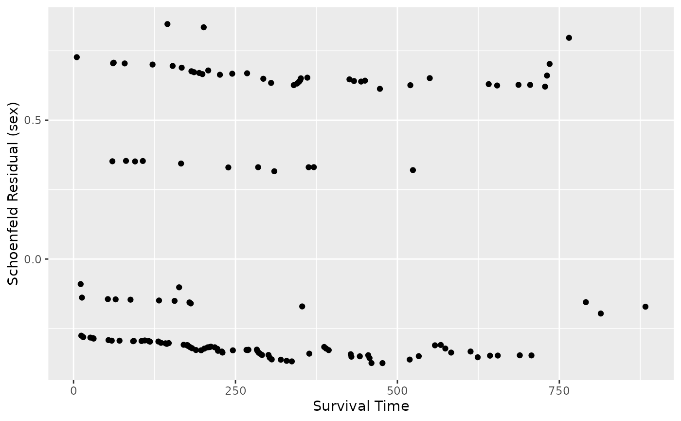
if (system.file(package = "ggplot2") != "") {
  g <- ggplot(res_sex, aes(x = .data$time, y = .data$y_scale)) +
    geom_point(color = "black") +
    labs(
      x = paste("Survival Time", sep = ""),
      y = paste("Schoenfeld Residual Scaled (sex)", sep = " ")
    )
} else {
  g <- message("ggplot2 wasn't detected. Please install to see the plot")
}
g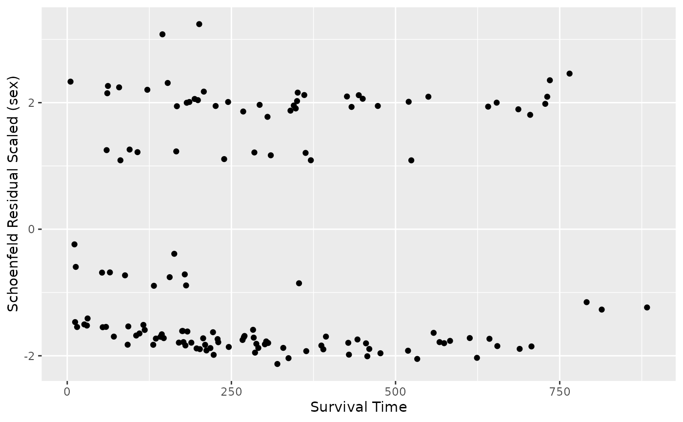
Martingale Residuals
Martingale residuals compare the event status and cumulative hazard for each subject. The residual is bound in the open interval . Negative residuals correspond with subjects that survive despite high cumulative hazard and residuals near unity correspond with subjects that experienced an event despite low cumulative hazard. The distribution of residuals with covariates can indicate if the model is over-predicting or under-predicting dependent on time.
We can plot martingale residuals using the
plotMartingale.coxres() function.
# We want to plot results by our two covariates
plot_options <- list(
  studyid = "UserID", verbose = 2,
  martingale = TRUE, cov_cols = c("age", "sex")
)
res_all <- plotMartingale(coxres, df, plot_options)
# We will have results for each covariate selected and the survival age.
res_age <- res_all[["age"]]

if (system.file(package = "ggplot2") != "") {
  g <- ggplot() +
    geom_point(
      data = res_age,
      aes(x = .data$cov_max, y = .data$res_sum, group = .data$event, color = .data$event)
    )
  g <- g + labs(x = "Max Age", y = "Martingale Residuals")
} else {
  g <- message("ggplot2 wasn't detected. Please install to see the plot")
}
g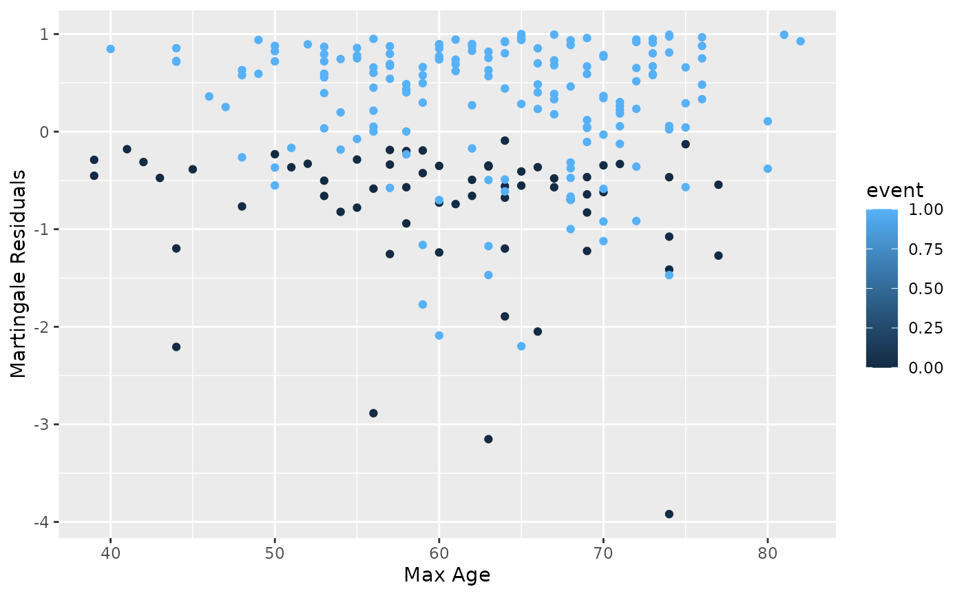
res_sex <- res_all[["sex"]]

if (system.file(package = "ggplot2") != "") {
  g <- ggplot() +
    geom_point(
      data = res_sex,
      aes(x = .data$cov_max, y = .data$res_sum, group = .data$event, color = .data$event)
    )
  g <- g + labs(x = "Sex", y = "Martingale Residuals")
} else {
  g <- message("ggplot2 wasn't detected. Please install to see the plot")
}
g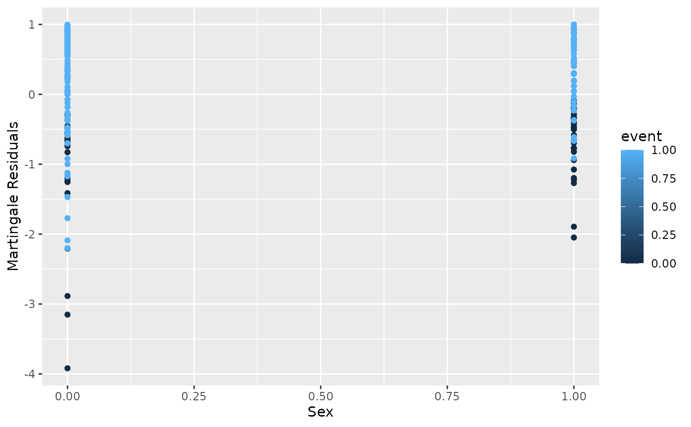
res_surv <- res_all[["survival_time"]]

if (system.file(package = "ggplot2") != "") {
  g <- ggplot() +
    geom_point(
      data = res_surv,
      aes(x = .data$time_max, y = .data$res_sum, group = .data$event, color = .data$event)
    )
  g <- g + labs(x = "Survival Time", y = "Martingale Residuals")
} else {
  g <- message("ggplot2 wasn't detected. Please install to see the plot")
}
g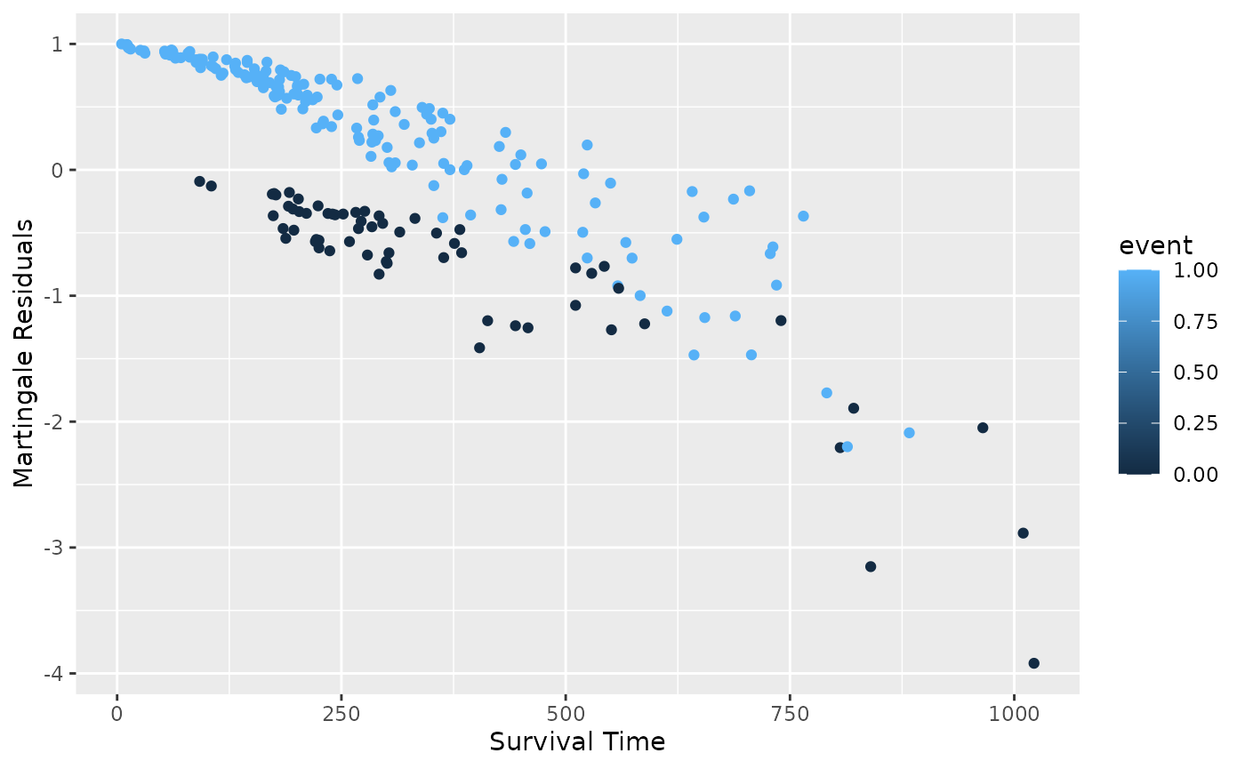
General Evaluation of Risk
Colossus also offers scripts that plot the relative risk
by covariate value for each covariate in the model, assuming every other
covariate is zero. Results for specific covariates can be requested by
passing an optional argument, otherwise every covariate used in the risk
model is included. Risk at Wald confidence interval boundaries can also
be calculated by including a ‘boundary’ option set to a z-score. In this
example, 95 percent confidence intervals are included and plotted. We
can plot the risk curves using the plotRisk.coxres()
function.
plot_options <- list(
  studyid = "UserID",
  verbose = 2, cov_cols = c("age", "sex"), boundary = 1.96
)
res_all <- plotRisk(coxres, df, plot_options)

res_age <- res_all[["age"]]

if (system.file(package = "ggplot2") != "") {
  g <- ggplot(res_age, aes(x = .data$x, y = .data$y)) +
    geom_errorbar(aes(ymin = .data$`y:lower`, ymax = .data$`y:upper`), color = "black") +
    geom_point(color = "black") +
    labs(x = "Age", y = "Relative Risk")
} else {
  g <- message("ggplot2 wasn't detected. Please install to see the plot")
}
g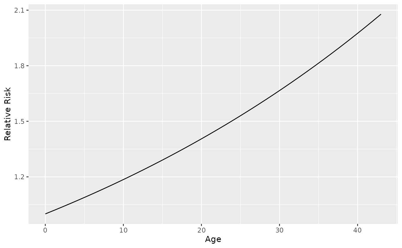
res_sex <- res_all[["sex"]]

if (system.file(package = "ggplot2") != "") {
  g <- ggplot(res_sex, aes(x = .data$x, y = .data$y)) +
    geom_errorbar(aes(ymin = .data$`y:lower`, ymax = .data$`y:upper`), color = "black") +
    geom_point(color = "black") +
    labs(x = "Sex", y = "Relative Risk")
} else {
  g <- message("ggplot2 wasn't detected. Please install to see the plot")
}
g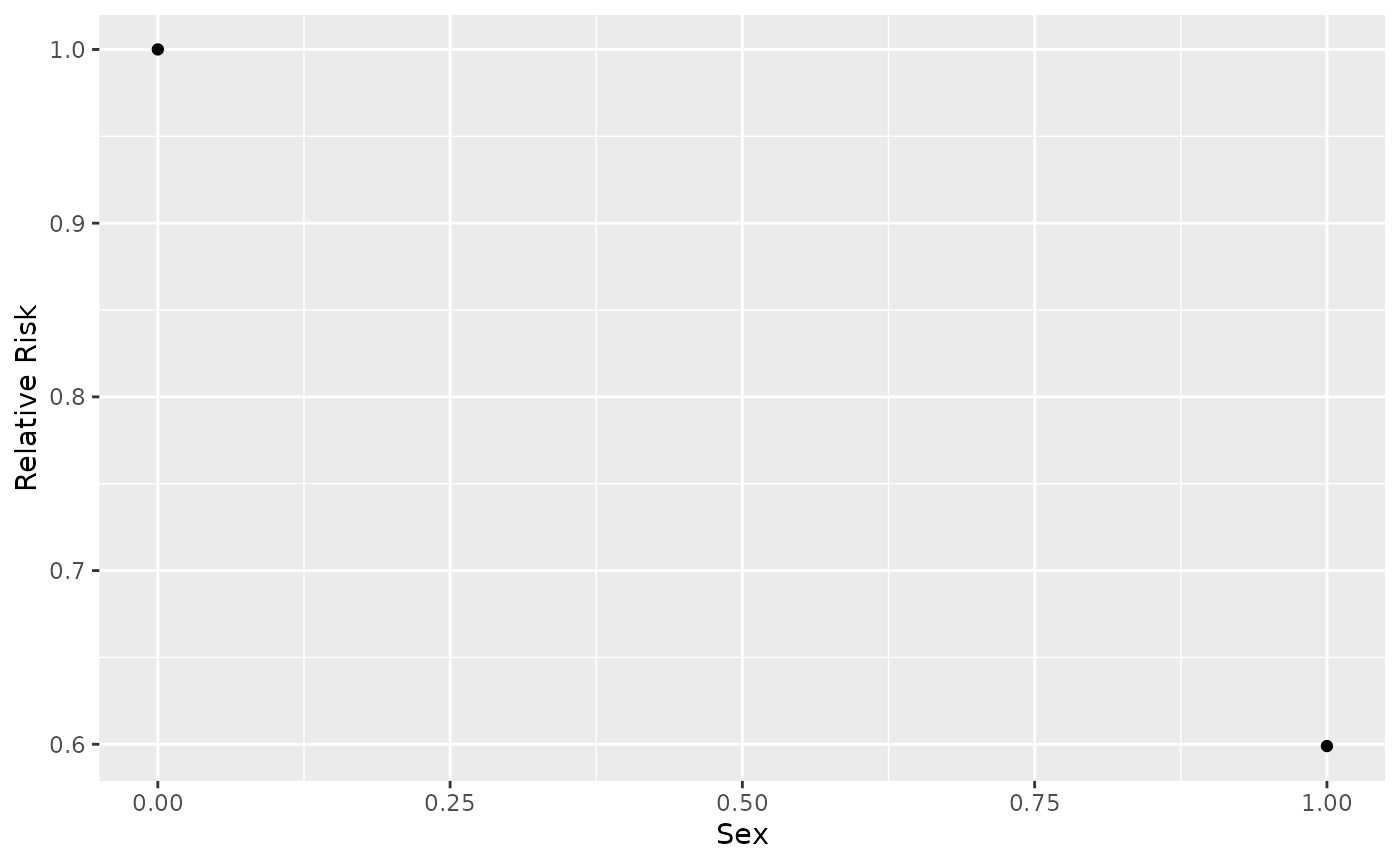
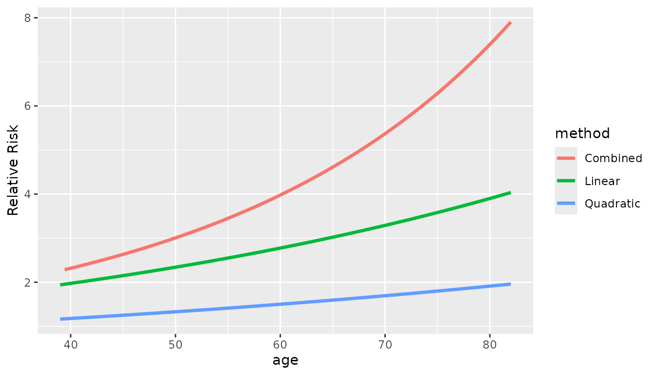
There is a similar option for returning predicted hazard ratio for a
set of input data points, or a reference point, called the
RelativeRisk.coxres() function. This can be used similarly
to the plotRisk() function by manually defining the points
to calculate risk at. This has one significant benefit, it can account
for interactions. If a model transforms a column, then it has multiple
covariates dependent on a single input column. The
plotRisk.coxres() function will only calculate the change
in risk based on the final calculated covariates independently, while
the RelativeRisk.coxres() function will properly account
for how each value depends on each other.
control <- list(ncores = 1)
a_n <- c(0.01701289, 0.0001, -0.51256478)
coxres <- CoxRun(Cox(time, status) ~ loglinear(age * age, sex, 0),
  df,
  control = control, a_n = a_n, norm = "max"
)
print(coxres)
#> |--------------------------------------------------------------------------------|
#> Final Results
#>    Covariate Subterm Central Estimate Standard Error 95% Confidence Interval
#>       <char>  <char>            <num>          <num>                  <char>
#> 1:       age  loglin           0.0170       0.112006    (-0.20252 - 0.23654)
#> 2:   age:age  loglin           0.0001       0.000901    (-0.00167 - 0.00187)
#> 3:       sex  loglin          -0.5126       0.167841    (-0.84153 - -0.1836)
#>    2-tail p-value
#>             <num>
#> 1:        0.87927
#> 2:        0.91160
#> 3:        0.00226
#> |- - - - - - - - - - - - - - - - - - - - - - - - - - - - - - - - - - - - - - - -|
#>
#> Cox Model Used
#> Survival Age Column was: 'time', Outcome Column was: 'status'
#> Risk Groups Used: 139
#> |- - - - - - - - - - - - - - - - - - - - - - - - - - - - - - - - - - - - - - - -|
#> -2*Log-Likelihood: 1487.827,  AIC: 1493.827
#> Iterations run: 3
#> maximum step size: 6.104e-05, maximum first derivative: 2.551e+00
#> Log-likelihood was not improved in last iteration
#> Analysis did not converge, step size limit was hit. Regression may converge if limit is reduced ('epsilon').
#> All Records Used: 228
#> Run finished in 0.047 seconds
#> |--------------------------------------------------------------------------------|
# There is a effect of age^2

# We can start by using plotRisk to calculate the effect of age

plot_options <- list(
  studyid = "UserID",
  verbose = 2, cov_cols = c("age", "age:age"), boundary = 1.96
)
res_all <- plotRisk(coxres, df, plot_options)
#> Warning in plot.coxres(x = x, df = df, plot_options = plot_options): Warning:
#> Columns were created during model defintion. Risk plots will only depend on
#> individual columns, not interactions

res_age <- res_all[["age"]]
res_age2 <- res_all[["age:age"]]

# We can also use a fake dataset and RelativeRisk
df_off <- df <- data.table(
  status = rep(0, 100),
  sex = rep(0, 100),
  time = rep(0, 100),
  age = (1:100) / 100 * (max(df$age) - min(df$age)) + min(df$age)
)

res_comb <- RelativeRisk(coxres, df_off)

# The same age values are used for each res_age x value, except the res_age2 is returning age^2
x_all <- c(res_age$x, res_age$x, df_off$age)
y_all <- c(res_age$y, res_age2$y, res_comb$Risk)
method <- c(rep("Linear", nrow(res_age)), rep("Quadratic", nrow(res_age2)), rep("Combined", nrow(df_off)))

comp_plot <- data.table(x = x_all, y = y_all, method = method)
# Plot them combined
if (system.file(package = "ggplot2") != "") {
  g <- ggplot(comp_plot, ggplot2::aes(x = .data$x, y = .data$y, group = .data$method, color = .data$method)) +
    geom_line(alpha = 1, linewidth = 1.2) +
    labs(x = "age", y = "Relative Risk")
} else {
  g <- message("ggplot2 wasn't detected. Please install to see the plot")
}
g