Sys.setenv(OMP_THREAD_LIMIT = 1) # Reducing core use, to avoid accidental use of too many cores
library(Colossus)
library(data.table)
if (system.file(package = "survival") != "") {
  library(survival)
}
library(dplyr)
#>
#> Attaching package: 'dplyr'
#> The following objects are masked from 'package:data.table':
#>
#>     between, first, last
#> The following objects are masked from 'package:stats':
#>
#>     filter, lag
#> The following objects are masked from 'package:base':
#>
#>     intersect, setdiff, setequal, union
General Usage
For Cox Proportional Hazards regression, the model is generally assumed to be independent of event time. However, for more complex models, Colossus can perform regressions using covariates that change over time. These can be split into two general types of covariates, step functions changing with time and multiplicative interactions with time. Colossus generates the new dataset by splitting each row of the original dataset into smaller intervals. This assumes that over each interval the values of every covariate are approximately constant. For Cox Proportional Hazards, rows that do not contain an event time are not used for regression, so Colossus has an option to only use small intervals around each event time. With this option, the time-dependent covariate is evaluated only at event times. For data-sets with a small number of discrete event times, this can save time and memory.
Multiplicative Interaction
The simplest type of time-dependent covariate is an interaction term between time and another covariate. Suppose we have a row in a dataset with a factor covariate “group” and some arbitrary endpoints to the time interval. Colossus starts by using a user-provided function to calculate the value of the time-dependent covariate at the endpoints. We assume that the value of “group” is constant over the interval and time is changing linearly. Colossus calculates the value of the time-dependent covariate over intervals by linearly interpolating between the values at the endpoints. This process assumes that the interaction is linear or the interval is small enough for the interaction to be approximately linear.
if (system.file(package = "ggplot2") != "") {
  dft <- data.table(x = c(1, 2, 3), y = c(2, 5, 10))
  g <- ggplot2::ggplot(dft, ggplot2::aes(x = .data$x, y = .data$y)) +
    ggplot2::geom_point(color = "black") +
    ggplot2::geom_line(color = "black", alpha = 1) +
    ggplot2::labs(x = "age (days)", y = "Covariate Value")
  x <- seq(1, 3, by = 0.1)
  y <- 1 + x^2
  dft <- data.table(x = x, y = y)
  g <- g + ggplot2::geom_line(
    data = dft, ggplot2::aes(x = .data$x, y = .data$y),
    color = "black", linetype = "dashed"
  )
} else {
  g <- message("ggplot2 wasn't detected. Please install to see the plot")
}
g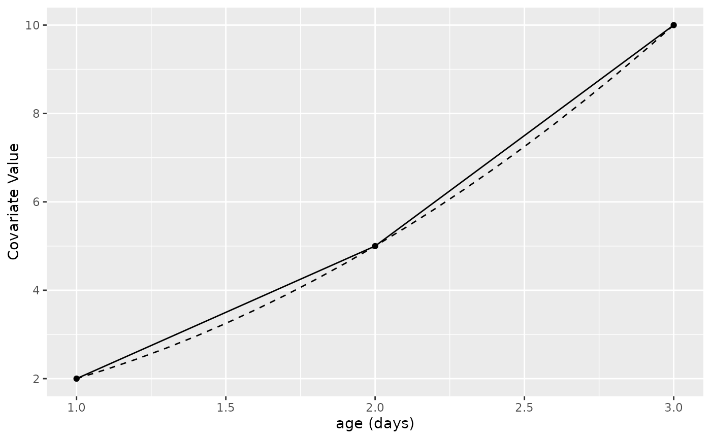
Linear Interpolated Function
This is most helpful in a situation where the user has continuous data over a series of intervals and believes that the values can be interpolated within each interval.
Step Function Interaction
The second type of time-dependent covariate changes based on conditional statements. One example is a covariate to split data into bins by time. Colossus uses a string to identify where to change value. The user inputs a string of the form “#l?” for a time value “#”, a condition “l”, and a question mark as a delimiter. Colossus allows for four conditions:
- l: less than or equal to
- g: greater than or equal to
- a: strictly above
- b: strictly below
So the following would be equivalent to “”
if (system.file(package = "ggplot2") != "") {
  dft <- data.table(x = c(-1, 1, 5, 8, 13), y = c(0, 1, 1, 2, 3))
  g <- ggplot2::ggplot(dft, ggplot2::aes(x = .data$x, y = .data$y)) +
    ggplot2::geom_point(color = "black")
  dft <- data.table(x = c(-1, -0.01, 0, 1, 5.99, 6, 11.99, 12, 13), y = c(0, 0, 1, 1, 1, 2, 2, 3, 3))
  g <- g + ggplot2::geom_line(data = dft, ggplot2::aes(x = .data$x, y = .data$y), color = "black") +
    ggplot2::labs(x = "age (days)", y = "Covariate Value")
} else {
  g <- message("ggplot2 wasn't detected. Please install to see the plot")
}
g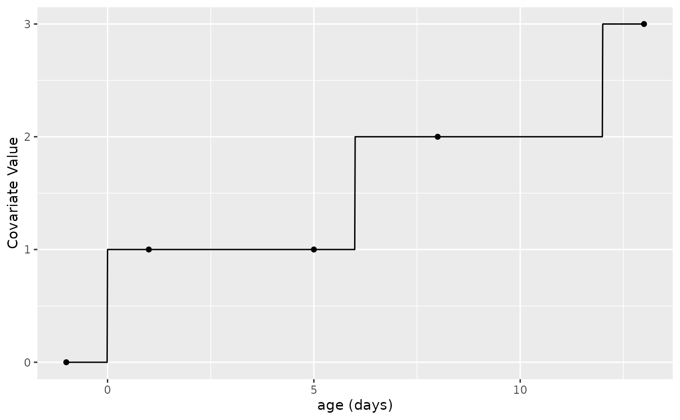
Monotonic Step Function Applied
Meanwhile the following is equivalent to “”
if (system.file(package = "ggplot2") != "") {
  dft <- data.table(x = c(-1, 1, 5, 8, 13), y = c(1, 2, 2, 3, 2))
  g <- ggplot2::ggplot(dft, ggplot2::aes(x = .data$x, y = .data$y)) +
    ggplot2::geom_point(color = "black")
  dft <- data.table(x = c(-1, -0.01, 0, 1, 5.99, 6, 11.99, 12, 13), y = c(1, 1, 2, 2, 2, 3, 3, 2, 2))
  g <- g + ggplot2::geom_line(data = dft, ggplot2::aes(x = .data$x, y = .data$y), color = "black") +
    ggplot2::labs(x = "age (days)", y = "Covariate Value")
} else {
  g <- message("ggplot2 wasn't detected. Please install to see the plot")
}
g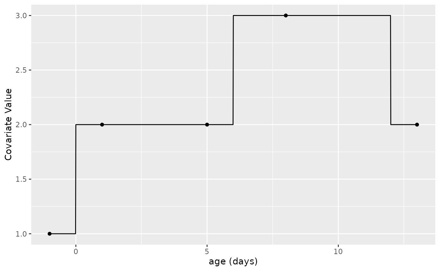
Step Function Applied
This is most helpful in situations where the user has reason to believe that the effect of a covariate on events is not uniform over time despite the covariate being constant over each interval. This allows the user to generate a list of factors to interact with any covariate of interest.
Examples of Use
The following provide a basic example for each method listed above. We start by setting up the data, which for this example is the cancer data from the R survival package.
# Setting up the data for use
if (system.file(package = "survival") != "") {
  data(cancer, package = "survival")
  cancer |> setDT()
  df <- copy(cancer)
} else {
  status <- c(2, 2, 1, 2, 2, 1, 2, 2, 2, 2, 2, 2, 2, 2, 2, 2, 2, 2, 2, 2, 2, 2, 2, 2, 2, 2, 2, 2, 2, 2, 2, 2, 2, 2, 2, 2, 2, 1, 2, 2, 2, 2, 2, 2, 2, 2, 2, 2, 2, 2, 2, 2, 2, 2, 2, 2, 2, 2, 2, 2, 2, 2, 2, 2, 2, 2, 2, 1, 2, 2, 1, 2, 2, 2, 2, 2, 2, 2, 2, 2, 2, 2, 1, 2, 1, 2, 2, 2, 1, 2, 2, 2, 2, 2, 1, 2, 2, 2, 2, 2, 1, 2, 2, 2, 2, 2, 1, 2, 2, 2, 2, 2, 2, 2, 2, 2, 2, 2, 2, 2, 2, 2, 2, 2, 2, 2, 2, 2, 1, 1, 2, 2, 2, 1, 2, 1, 2, 2, 2, 2, 2, 1, 2, 2, 1, 1, 2, 2, 2, 2, 2, 1, 1, 2, 2, 2, 1, 2, 2, 1, 1, 2, 1, 2, 1, 1, 2, 2, 2, 2, 1, 2, 2, 1, 1, 1, 2, 2, 2, 1, 1, 1, 2, 1, 1, 1, 2, 1, 2, 2, 2, 2, 2, 1, 2, 1, 1, 1, 1, 2, 2, 2, 1, 1, 1, 2, 1, 2, 1, 1, 1, 1, 1, 1, 2, 1, 1, 2, 1, 1, 1, 1, 2, 1, 1, 1, 1, 1)
  sex <- c(1, 1, 1, 1, 1, 1, 2, 2, 1, 1, 1, 2, 2, 1, 1, 1, 1, 1, 2, 1, 1, 2, 1, 1, 1, 2, 1, 1, 1, 1, 2, 1, 1, 2, 1, 2, 1, 2, 1, 2, 1, 2, 2, 2, 1, 2, 1, 1, 1, 2, 2, 1, 1, 1, 1, 1, 2, 1, 2, 2, 2, 1, 1, 2, 1, 1, 2, 2, 1, 1, 1, 2, 1, 1, 2, 2, 2, 2, 1, 1, 1, 1, 1, 2, 1, 1, 2, 1, 2, 1, 1, 1, 1, 2, 2, 1, 1, 1, 1, 2, 2, 2, 1, 1, 1, 1, 2, 1, 1, 2, 1, 1, 1, 2, 2, 1, 1, 1, 1, 1, 1, 2, 2, 1, 1, 1, 1, 1, 2, 2, 2, 1, 1, 2, 1, 2, 2, 1, 1, 1, 2, 1, 1, 2, 1, 2, 1, 1, 1, 2, 1, 1, 2, 2, 1, 1, 2, 1, 1, 2, 2, 2, 1, 1, 1, 2, 2, 1, 1, 1, 1, 2, 1, 2, 1, 2, 1, 2, 2, 2, 1, 1, 2, 2, 2, 2, 2, 1, 1, 1, 1, 1, 1, 1, 1, 1, 2, 1, 2, 1, 2, 1, 2, 2, 2, 1, 2, 2, 1, 2, 2, 1, 1, 2, 1, 1, 2, 1, 2, 2, 1, 2, 1, 1, 1, 2, 1, 2)
  time <- c(306, 455, 1010, 210, 883, 1022, 310, 361, 218, 166, 170, 654, 728, 71, 567, 144, 613, 707, 61, 88, 301, 81, 624, 371, 394, 520, 574, 118, 390, 12, 473, 26, 533, 107, 53, 122, 814, 965, 93, 731, 460, 153, 433, 145, 583, 95, 303, 519, 643, 765, 735, 189, 53, 246, 689, 65, 5, 132, 687, 345, 444, 223, 175, 60, 163, 65, 208, 821, 428, 230, 840, 305, 11, 132, 226, 426, 705, 363, 11, 176, 791, 95, 196, 167, 806, 284, 641, 147, 740, 163, 655, 239, 88, 245, 588, 30, 179, 310, 477, 166, 559, 450, 364, 107, 177, 156, 529, 11, 429, 351, 15, 181, 283, 201, 524, 13, 212, 524, 288, 363, 442, 199, 550, 54, 558, 207, 92, 60, 551, 543, 293, 202, 353, 511, 267, 511, 371, 387, 457, 337, 201, 404, 222, 62, 458, 356, 353, 163, 31, 340, 229, 444, 315, 182, 156, 329, 364, 291, 179, 376, 384, 268, 292, 142, 413, 266, 194, 320, 181, 285, 301, 348, 197, 382, 303, 296, 180, 186, 145, 269, 300, 284, 350, 272, 292, 332, 285, 259, 110, 286, 270, 81, 131, 225, 269, 225, 243, 279, 276, 135, 79, 59, 240, 202, 235, 105, 224, 239, 237, 173, 252, 221, 185, 92, 13, 222, 192, 183, 211, 175, 197, 203, 116, 188, 191, 105, 174, 177)
  age <- c(74, 68, 56, 57, 60, 74, 68, 71, 53, 61, 57, 68, 68, 60, 57, 67, 70, 63, 56, 57, 67, 49, 50, 58, 72, 70, 60, 70, 53, 74, 69, 73, 48, 60, 61, 62, 65, 66, 74, 64, 70, 73, 59, 60, 68, 76, 74, 63, 74, 50, 72, 63, 68, 58, 59, 62, 65, 57, 58, 64, 75, 48, 73, 65, 69, 68, 67, 64, 68, 67, 63, 48, 74, 40, 53, 71, 51, 56, 81, 73, 59, 55, 42, 44, 44, 71, 62, 61, 44, 72, 63, 70, 66, 57, 69, 72, 69, 71, 64, 70, 58, 69, 56, 63, 59, 66, 54, 67, 55, 75, 69, 44, 80, 75, 54, 76, 49, 68, 66, 80, 75, 60, 69, 72, 70, 66, 50, 64, 77, 48, 59, 53, 47, 55, 67, 74, 58, 56, 54, 56, 73, 74, 76, 65, 57, 53, 71, 54, 82, 59, 70, 60, 62, 53, 55, 69, 68, 62, 63, 56, 62, 44, 69, 63, 64, 57, 60, 46, 61, 65, 61, 58, 56, 43, 53, 59, 56, 55, 53, 74, 60, 39, 66, 65, 51, 45, 72, 58, 64, 53, 72, 52, 50, 64, 71, 70, 63, 64, 52, 60, 64, 73, 63, 50, 63, 62, 55, 50, 69, 59, 60, 67, 69, 64, 65, 65, 41, 76, 70, 57, 67, 71, 76, 77, 39, 75, 66, 58)

  df <- data.table(
    status = status,
    sex = sex,
    time = time,
    age = age
  )
}

df$UserID <- seq_len(nrow(df))

df$status <- df$status - 1
df$sex <- df$sex - 1

t0 <- "%trunc%"
t1 <- "time"
event <- "status"

df <- df[, c("time", "status", "sex", "UserID")]
For the first example we will linearly interpolate the product of time and biological sex.
grt_f <- function(df, time_col) {
  (df[, "sex"] * df[, get(time_col)] / 400)[[1]]
}
func_form <- c("lin")
iscox <- TRUE
dt <- 0.01
df_new <- gen_time_dep(
  df, t0, t1, event, iscox, dt, c("sex_time"), c(),
  c(grt_f), paste0(tempfile(), "test_new.csv"), func_form,
  nthreads = 1
)
if (system.file(package = "ggplot2") != "") {
  g <- ggplot2::ggplot(df_new, ggplot2::aes(x = .data$time, y = .data$sex_time, colour = factor(.data$sex))) +
    ggplot2::geom_point() +
    ggplot2::geom_line() +
    ggplot2::labs(x = "Time", y = "Covariate Value")
} else {
  g <- message("ggplot2 wasn't detected. Please install to see the plot")
}
g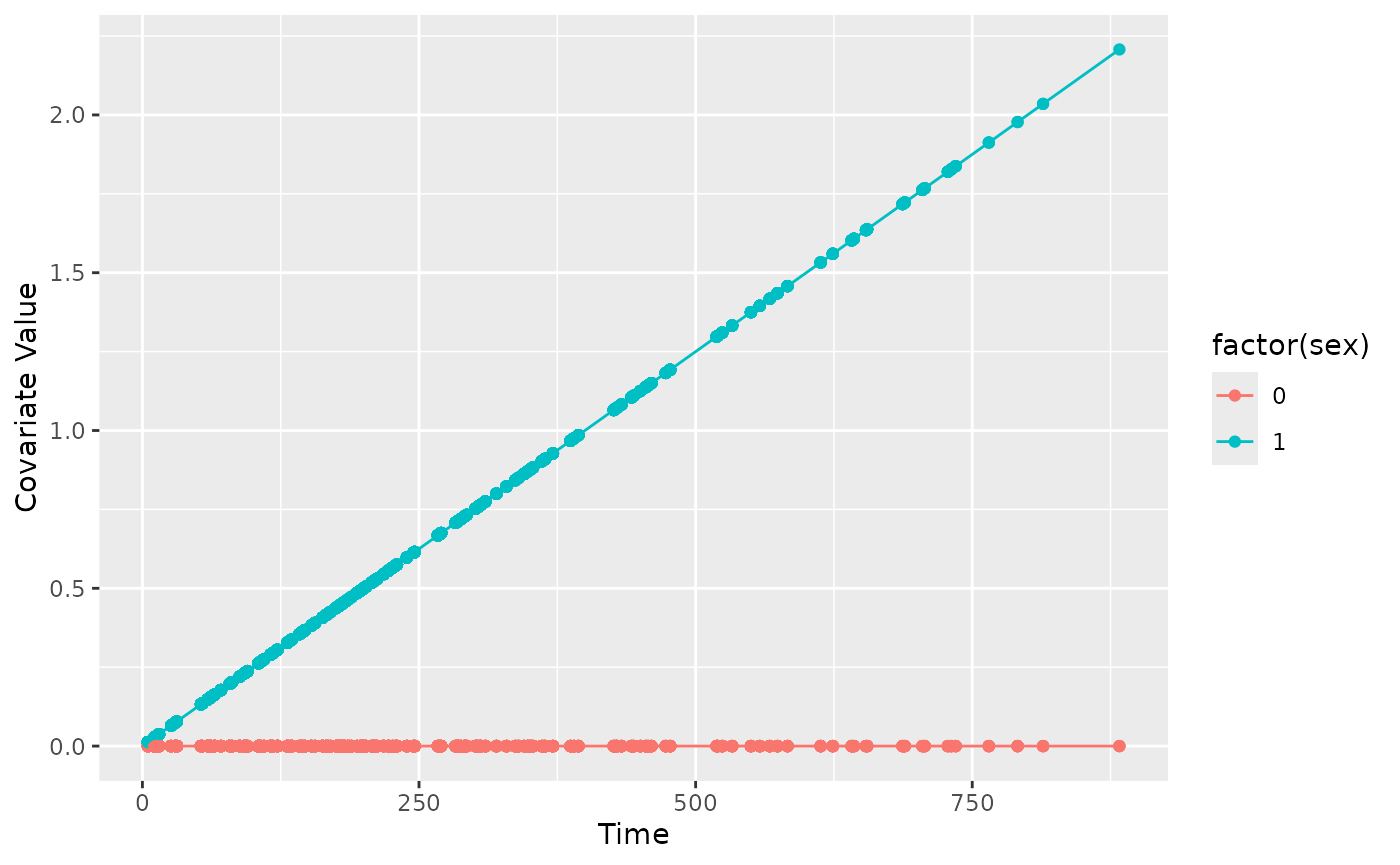
Linear Interpolation Example
For the second example we will use a step functions that increases at 200, 500, and 700 days.
func_form <- c("step?0g?200g?500g?700g?")
df_new <- gen_time_dep(
  df, t0, t1, event, iscox, dt, c("time_step"), c(),
  c(grt_f), paste0(tempfile(), "test_new.csv"), func_form,
  nthreads = 1
)
if (system.file(package = "ggplot2") != "") {
  g <- ggplot2::ggplot(df_new, ggplot2::aes(x = .data$time, y = .data$time_step)) +
    ggplot2::geom_point(color = "black") +
    ggplot2::geom_line() +
    ggplot2::labs(x = "Time", y = "Covariate Value")
} else {
  g <- message("ggplot2 wasn't detected. Please install to see the plot")
}
g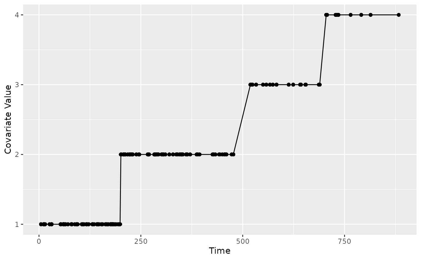
Monotonic Step Function Example
For the third example we will use a step functions that increases at 200, 400, and 700 days and decreases at 600 and 800 days.
func_form <- c("step?0g?200g?400g?600l?700g?800b?")
df_new <- gen_time_dep(
  df, t0, t1, event, iscox, dt, c("time_step"), c(),
  c(grt_f), paste0(tempfile(), "test_new.csv"), func_form,
  nthreads = 1
)
if (system.file(package = "ggplot2") != "") {
  g <- ggplot2::ggplot(df_new, ggplot2::aes(x = .data$time, y = .data$time_step)) +
    ggplot2::geom_point(color = "black") +
    ggplot2::geom_line() +
    ggplot2::labs(x = "Time", y = "Covariate Value")
} else {
  g <- message("ggplot2 wasn't detected. Please install to see the plot")
}
g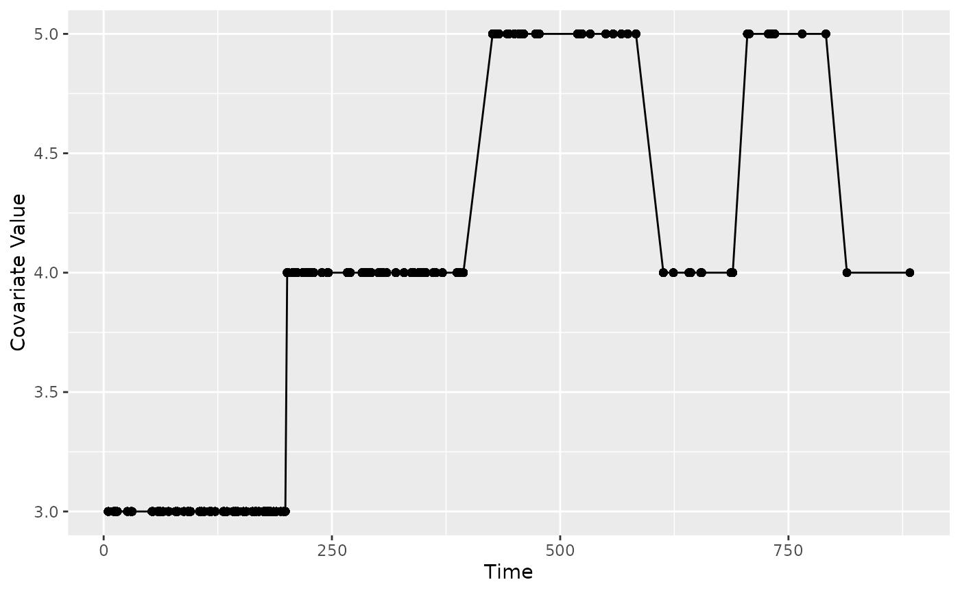
Step Function Example